Semantic Segmentation
Warning
This section is very much work in progress!
Semantic segmentation also known as pixel-level classification, is a pixel-level classification of images. The generated segmented map can be a resampled to spacial representation of the input image. Semantic segmentation can also be extended to localize the object in computer vision problems.
In the context of document image analysis, semantic segmentation can be referred to as document image binarization, where the pixels in the image are represented as either background class or foreground class where background class is represented as black pixel and background pixel is represented as a white pixel.
Fully convolution networks
Fully convolution networks (FCN) are elegant forms of typical convolution networks that do not use any fully connected layers after the convolution layers to output a non-spacial label for a given input image. Unlike the other deep neural networks, FCNs can be trained on images of arbitrary sizes to make a pixel-level prediction i.e. FCNs can be leveraged to form inference between the input image and output image on pixel-level.
FCNs are different from the other image classification algorithms in a way that the FCNs can output spacial and possibly resampled outputs to the input image, instead of a non-spacial label. This ability to generate spacial output makes the FCNs suitable for semantic segmentation. Deeply connected convolution layers are used to extract global level and local level features from the input images. The global level features refer to what and local level features gives the idea of where in the context of image features. The input image dimensions are reduced by subsampling and reduced to a lower level dimension, which, in a way, represents the cost function of the task we are performing. The dimensions are reduced to keep the convolution layer kernels small and reduced the computations to a reasonable size. The output maps are then mapped to real pixel values using upsampling, which is also known as deconvolution.
U-net
U-net is a U shaped fully convolution network, which has a contraction path and an upsampling path with the convolution layers in both the paths more or less have a symmetry to each other. U-net architecture is designed such that it can give better segmentation maps even with very few input images.
Pooling layers in the FCNs are replaced by upsampling layers where the high-level features from the contracting path are combined with upsampled output. Instead of interpolating the features, the high-level features are then given to the convolution layer to learn and from a more precise output based on this information. A large number of feature channels in the upsampling path allows the network to propagate more contextual information to the higher resolution layers.
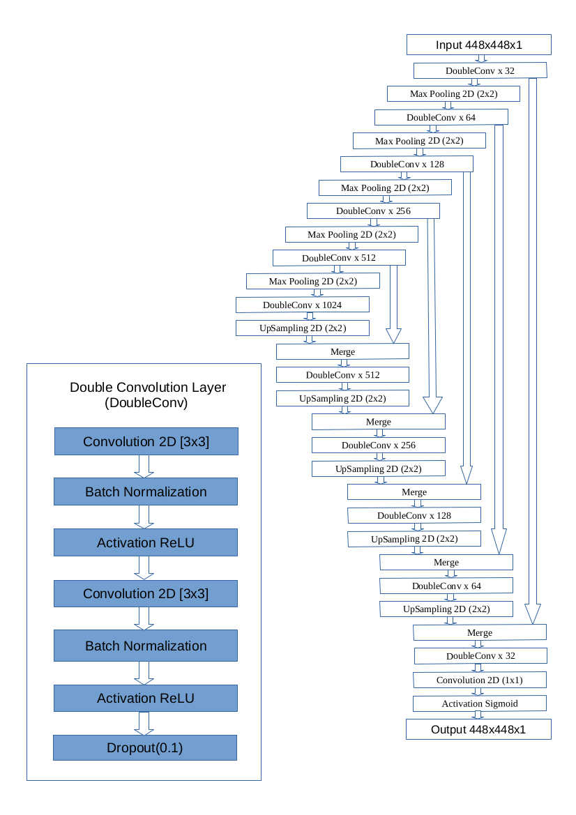
Figure: U-net architecture used in UNAGI.
The original U-net architecture is modified by adding batch normalization after each convolution layer and dropout layer at the end of the double convolution layer. A double convolution layer with a dropout of 10% is used after each double convolution layer. The upper part of the architecture is a contracting path where each convolution layer is followed by a ReLU activation layer and a 2 ∗ 2 max pooling op- eration with stride 2 for downsampling the features. At each downsampling stage, feature channels are doubled, and at the upsampling part, the feature maps are halved, followed by an up-convolution/deconvolution layer. At the final layer, a 1 ∗ 1 convolution is used to map each feature vector to the desired number of classes. In total, the network has 23 convolutional layers.
Evaluation metrics
The neural network predictions can be evaluated with the accuracy in image classification. However, accuracy might not be the most suitable quantitative metric to measure the model performance. In the context of semantic segmentation, similarity measures such as the Dice coefficient and Jaccard coefficients can be used to measure the similarity between the input image and predicted segmentation mask.
Binary accuracy
Accuracy in semantic segmentation can be calculated as the percentage of pixels that are classified correctly in the total number of pixels. Binary classification in terms of true positive (TP), false positive (FP), false negative (FN) and true negatives can be calculated as,
Accuracy can be a misleading metric if there is a high-class imbalance, where one class has more presence than the other class. This would not give the correct accuracy of the negative class.
Dice coefficient
Given two sets A and B, the Dice similarity coefficient of the two sets is equal to twice the number of elements common in both sets to the total number of elements in both sets.
Where \(A_n\) and \(B_n\) are the total number of elements in set A and set B, respectively. The dice coefficient of two binary entities can be calculated by considering fore- ground and background classes as two sets with the elements. When applied to two binary vectors, using the definition of true positives (TP), false positive (FP), and false-negative (FN), the Dice coefficient can be written as,
Loss functions
Loss functions for semantic segmentation tasks should be able to deal with class imbalance. It is often the case that there exists a huge class imbalance while training a semantic segmentation model. Especially in the context of text binarization, there are two classes, one being the background and other being foreground. The foreground class should contain text, and background should contain while pixels. When compared with the number of background pixels, foreground text pixels are very less, which leads to a huge class imbalance.
Weighted cross-entropy loss
Weighted cross-entropy loss is derived from the cross-entropy loss. Cross entropy, in general, represents the distance between the true distribution and predicted distribution of the neural network model. Binary cross-entropy is considered when the number of classes is two. Cross entropy is calculated for all the data points in the training dataset, and the average of both positive and negative classes is calculated to get the final loss value.
Cross entropy loss function can be extended by adding a weight balancing factor α ∈ [0, 1] to the loss function, where α is the weight factor for positive class and 1 − α is the weight factor for the negative class.
Where p ∈ [0, 1] is the probability of predicted value and y ∈ {±1} is the ground truth value.
Focal loss
Focal loss, derived from weighted cross-entropy, has two main advantages where the loss can be used to deal with huge class imbalance problems and overwhelming problem. The overwhelming problem can be present in a semantic segmentation problem where easily classified samples from negative class drive the gradient. Focal loss is modified from weighted cross-entropy to differentiate the easy and hard samples in the data and down weight the easy samples so that the hard samples can have more weightage during loss calculation. A modulating factor with a tunable focusing factor γ ≥ 0 is added to the cross-entropy loss to define the focal loss. Weight balanced focal loss can be described as,
Where \(p_t\) is
Where p ∈ [0, 1] is the probability of predicted value and y ∈ {±1} is the ground truth value.
Dice loss
Dice loss is extended from the Dice similarity coefficient that is used to measure the overlap between segmented maps in semantic segmentation. Dice loss is used to minimize the overlap between the predicted segmentation map and original segmentation map.
Where \(DSC_c\) is the Dice similarity coefficient Although dice loss being one of the most used losses in semantic segmentation, it has a drawback of equally weighting the false negatives (FN) and false positives (FP).
Focal Tversky loss
Focal Tversky loss is a combination of both the Tversky index and focal loss. Focal Tversky loss is designed to address highly imbalanced data with a small region of interests(ROIs) such as skin lesions or characters on document images. Small ROIs contribute very little to the loss function. This lead to the misclassification of these small regions. False negatives(FNs) need to be weighted higher during the loss calculation than false positives(FPs) to improve the detection of class with less number of samples. Focal Tversky loss with a modulating factor \(\gamma\) can be described as:
Where \(TI_c\) is the Tversky index,
Where \(\alpha\) is the weight factor to use on false positives, \(\beta\) or (1-\(\alpha\)) is the weight factor used on false negatives and \(\epsilon\) is the constant that is added to both nominator and denominator for mathematical flexibility.
If \(\gamma > 1\), the loss function will focus more on pixels with less prediction probability. \(\gamma\) usually varies in the range [1,3]. FTL is unaffected when a pixel is wrongly classified with high Tversky index, but if the pixel is wrongly classified with less Tversky index, the Focal Tversky loss will be decreased.