Artificial Neural Networks
Warning
This section is very much work in progress!
Artificial neural networks (ANNs), or as they commonly referred to as neural networks, are machine learning models designed after the biological neurons in the human brain. These neural networks act as an approximation function based on inputs.
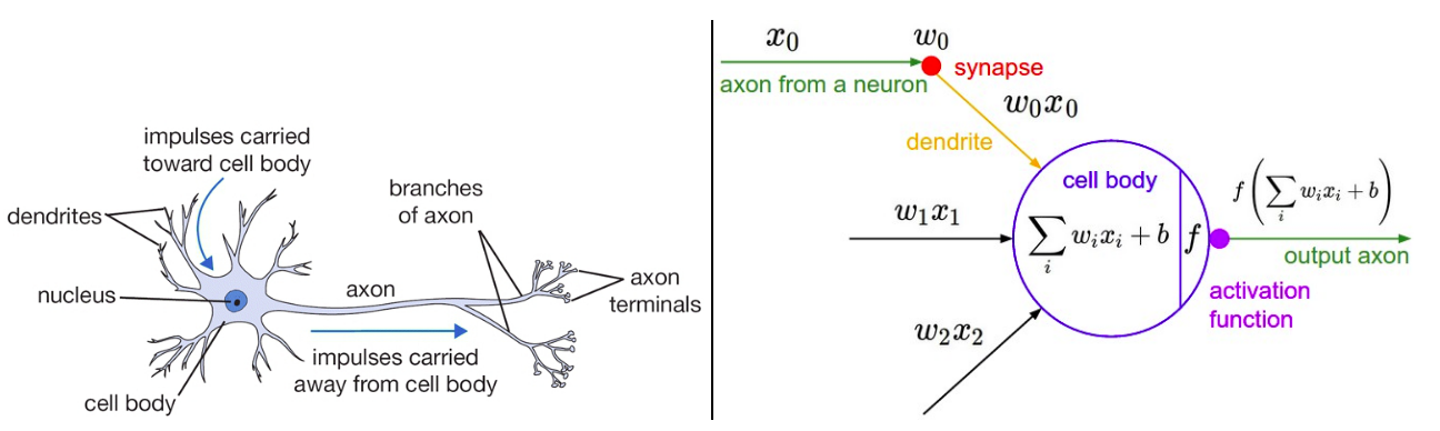
Figure 1: Biological neuron (left) and it’s mathematical representation (right).
The original neural network, called as a perceptron, was designed in 1958. A perceptron is a simple model that has only two layers, input layer and an output layer with a simple activation function based on sum and multiplication. These simple models can only learn linearly separable functions. Non-linear function approximations are learned by adding hidden layers to the model. Neural networks with hidden layers are commonly referred to as multi-layer perceptrons (MLPs). A sufficiently large MLP with many hidden layers could act as a universal approximator, which can approximate any type of function. These models are also called as feedforward neural networks.
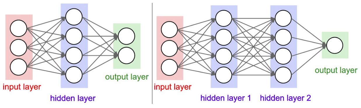
Figure 2: (Left) Neural network with one hidden layer and two output neurons in ouput layer. (Right) Neural network with two hidden layers and one output neuron in ouput layer.
These models are called feedforward because information flows through the function being evaluated from x, through the intermediate computations used to define f, and finally to the output y. There are no feedback connections in which outputs of the model are fed back into itself. When feedforward neural networks are extended to include feedback connections, they are called recurrent neural networks.
Training data
The resurgence of neural networks was mainly due to the explosion of the internet in the past decade. Training neural networks needs a lot of input data. Preparing data to train a neural network can be a costly, time consuming, and tedious task sometimes. Data is prepared in 3 subsets to train a neural network.
Train data: Train data acts as input data to train the actual model. Each sample in the train data set acts as input to the input layer of the network, and the learning algorithm learns the output of the corresponding input sample. Each time the network trains on all the given train data samples, one epoch of training finishes. It is common practice to train a neural network for more than one epoch.
Validation data: Validation data acts as test data to measure the learning process on unseen data while the training is ongoing. The learned approximation function tests the validation data at the end of every epoch, and the error calculated from the validation data, also called validation error, acts as a measure while updating the approximation function further. Validation data should not contain any samples from either train data or the test data.
Test data: The learned function is tested on a never seen data at the end of training to see how well the model can perform on new data that was not available during the training or validation of the network. The test error rate calculated on the test data gives an idea of how well the trained network can perform on new data. The model has a high generalization ability if the error rate is less for test data.
Class imbalance
Class imbalance in the context of machine learning occurs in the data when there is a huge difference in the number of samples present in each class. Having a class imbalance in the data would lead to the neural network model to predict the class with a higher number of samples more often. Measuring the goodness of a neural network model can be tricky when there is a huge class imbalance since the model will predict the highest class more often than the other classes. Each class can have class weights while calculating the loss value during backpropagation to address the class imbalance in the data.
Batchsize
Batchsize or mini batchsize is the number of samples that are used to calculate the error that is propagated back to the input layer from the output layer. The input layer in the neural network receives the number of inputs based on the batchsize. Batchsize can vary from 1 to any multiple of 2. Usually, it is preferred to have a batchsize, which is a multiple of 2 for the ease of computation. Choosing batch size also depends on the amount of computation memory available.
Small batches can offer a regularizing effect, perhaps due to the noise they add to the learning process. Generalization error is often best for a batch size of 1. Training with such a small batchsize might require a small learning rate to maintain stability because of the high variance in the estimate of the gradient. The total runtime can be very high as a result of the need to make more steps, both because of the reducedlearning rate and because it takes more steps to observe the entire training set.
Learning rate
A loss function is used to optimize the parameters of neural networks. Weights of the neural network are optimized using SGD to minimize the loss calculated from loss function. The loss value is calculated by using loss function by approximating the predicted value with the actual output value. The loss function selection for a neural network model depends on the task.
Activation function
The ability of neural networks to approximate any function, especially the non- convex function, is mainly due to their non-linear activation functions. An activa- tion function takes a vector as an input and performs a piece-wise operation on it, which in turn adds non-linearity to the liner outputs of individual neurons outputs.
Regularization
A deep learning model should be able to generalize well on unseen data. The test error of a deep learning model is a measure to estimate the generalization ability of the model. Test error is also known as generalization error. If a model is not performing well on unseen data, there can be two reasons for it, the model does not have the capacity and underfits the function that is being approximated, or the model is closely fitted to the training data and overfits the function. If a model underfits, both training error and test error will be less, and if the model overfits the data, the training error will be less, and the test error will be very high. A well performing deep leaning model should have a low test/generalization error. Regularization is a method to reduce the generalization error. Proper regularization of a deep learning model could result in the best-fitting model.
Data argumentation
One way to improve the results of any learning model is to train it with more data so that it can learn from more examples. Creating fake or simulated data from the training data has become a reliable practice in training a deep learning model. This process is called data argumentation. Data argumentation lets us train with more data with minimal effort to create new data. There exist two methodologies to perform data argumentation. One is to create simulated data before starting the model training, and the other is creating the data during the model training. The second method gives the option to save the data preparation time and space to save the data.
Batch Normalization
The basic idea of training a deep learning model with batch normalization is to limit the change in the distribution of input to all the layers in the network. The effect of having different distributions of data for input is known as the covariate shift. Batch normalization transforms the input activation to have zero mean and unit variance. This effect allows the network to have a more stable distribution of inputs throughout the network and thus allowing the network to train faster. Batch normalization also lets the network to train with higher learning rates to further improve the convergence speed of the network. Different elements of the same feature map need to be normalized in the same to follow the convolution property, due to this, all the activations in a batch is normalized jointly in all places.
Dropout
Dropout is a powerful regularization yet easy to implement regularization method. Dropout trains the model by removing the nonoutput units from the underlying network layers. Dropout lets the model train with fewer nodes than the number of nodes that are available for training so that the network can choose to learn more significant features extracted from the image. Dropout makes the model forget the features which are sometimes specific to certain data points. Using dropout forces the model to figure out more general features from the images. The number of units not used while training the model will be available during the model prediction. Dropout could cause the model to perform well in the initial stage of training, which could result in having lower validation error then the training error which will catch up after few epochs.
Earlystopping
When training large deep learning models which leads to overfitting of the data, it can be observed that the training error and validation error decreases gradually, and at some point, the validation error will start to increase. This means the best fitting model is already available. Early stopping is a method to stop training the model if the model meets certain criteria such as, reaching a particular value for validation error or if it does not improve for some epochs.
Along with training the model until the model meets this criterion, the best model parameters are saved at each epoch when improved from the previous best parameters with lowest loss value at a certain epoch. This might take some space and time to perform the IO operation of saving these model parameters, but this is negligible when compared to the time it is required to train a deep learning model. Early stopping needs validation data, which means the model is not trained with all the data available. Once the training is finished with early stopping, the model can be trained again with all the data until the model reached the lowest validation error observed early stopping. Another way is to continue training the model by using the previously saved best model parameters and full training data.
Note
Figure 1 and 2 are taken from CS231