Optimization of Nerual Networks
Warning
This section is very much work in progress!
Most deep learning algorithms involve optimization of some sort. Optimization refers to the task of either minimization or maximization of some function \(f(x)\) by changing \(x\). The function we want to minimize or maximize is called objective function. When minimizing it, it may be referred as cost funciton, loss function, or error funciton.
Loss function
A loss function measures how compatible given a set of parameters is with respect to the ground truth labels. The loss function is defined in such a way that making good predictions on the training data should result in a small loss. Weights of the neural network are optimized using SGD to minimize the loss calculated from loss function. The loss value is calculated by using loss function by approximating the predicted value with the actual output value. The loss function selection for a neural network model depends on the task.
Suppose we have a function \(y=f(x)\), where both x and y are real numbers. The derivative of this function is denoted as \(f'(x)\) and it specifies how to scale a small change in the input to obtain the corresponding change in the output. The derivative is useful in minimizing a function becasue it tells us how to change \(x\) in order to make a small improvement in \(y\). The function \(f(x)\) can be reduced by moving \(x\) in small steps with respect to the derivative. This technique is called as gradient descent.
Gradient based optimization
Optimization algorithms that use only sub set of entire training set are called as minibatch stochastic methods or simply stochastic methods. Although Stochastic gradient descent (SGD) means that the minibatch size should be 1, it is commonly choose it from one to few hundred. The insight of SGD is that the gradient is an expectation and the expectation is estimated on minibatch insterd of on full training set. Compting the gradient on minibatch is less computationally expensive compared to the entire dataset. The loss function is optimized with iterative refinement of gradient which also gives the steepest ascent direction. The gradient tells us the direction in which the function has the steepest rate of increase, but it does not tell us how far along this direction we should step.
A hyperparameter called step size (or learning rate) is used to make these steps in the given direction. Small steps are likely to lead to consistent but slow progress. Large steps can lead to better progress but are more risky. Note that eventually, for a large step size we will overshoot and make the loss worse. The step size is one of the most important hyperparameter that one have to carefully tune.
When dealing with optimization of funciton with multidimentional inputs, finding globel minima might not be possible, so we can settle for a local minima whcih is close to the globel minima but not a local minima.
Critical points/stationary points: The points where the derivative is 0. In such case it can not provide the information about which direction to move the \(x\).
Local minimum: A point where \(f(x)\) is lower than all neighboring points os that it is no longer possible to decrease \(f(x)\).
Local maximum: A point where \(f(x)\) is higher than all neighboring points os that it is no longer possible to decrease \(f(x)\).
Saddle points: A critical point which is either minimum or maximum.
Globel minimum: A point that obtains the absolute lowest value of \(f(x)\). There can be more than one globel minima of a function.
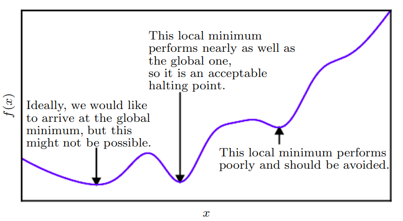
Figure 1: Selection of minima which gives the lowest value for loss funciton.
Vanishing gradients: Occures when the gradient is vanishingly small which will basically not change the weight value.
Exploding gradients: Error gradients can accumlate during an update and results in large gradinets and weights updations.
Vanishing gradients make it difficult to know which direction the parameters should move to improvethe cost function, while exploding gradients can make learning unstable. This can be avoided by using gradient clipping while updating the weights. This will make a change to the step size accordingly so that the loss funciton does not move too far or too less in the praposed direction.
Backpropagation
The gradients which are used to updated the weights are calculated using a method called backpropagation. It is the most used method to compute gradients, often used along with SGD to optimize neural networks.
Gradients are calculated by taking partial derivatives of the function. These gradients are chained together by following the chain rule of caclulas. The chain rule tells us the correct way to chain these gradients expressions together through multiplication. Backpropagation allows us to effictly calculate gradients of loss functions with respect to it’s parameters. For example if \(f(x,y,z) = (x+y)z\) is a simple function of variables \(x,y,z\) then the gradient variables (the partial derivatives) \(\frac{df}{dx},\frac{df}{dy},\frac{df}{dz}\) will tell us the sensitivity of the variables \(x,y,z\), on the function \(f\).
For any neural netwotk which uses backpropagation to calculate the gradients, the gradients are calculated during both forward pass and backward pass. During forward pass, gradients are computed from inputs to outputs and during backward pass backpropagation is performed which starts at the output and recursively applies the chain rule to compute the gradients all the way back to the inputs of the network. Once the forward pass is over, during backpropagation the gate will eventually learn about the gradient of its output value on the final output of the entire circuit. Chain rule says that the gate should take that gradient and multiply it into every gradient it normally computes for all of its inputs. The loss function is then moved towards the lowest value based on the direction that gradient provides using the step size provied.
Note
Figure 1 is taken from Deep Learing Book